The Role of Neural Networks in Generative Models

Generative AI is an immensely popular topic. We have seen many new models coming out the last few years. These models generate impossibly high quality samples in almost all digital media: text, images, speech, and music. This blog post takes a look at how some of these models are formulated. I focus on making it obvious how neural networks are used as the key technique to approximate the most intractable components. My goal is to demystify these generative models, and empower distributed system engineers to dig deeper and become comfortable contributing to writing high performance codes for inference and training of AI models.

Neural Networks as Approximations

A neural network is a parametrized function. A linear regression is a parametrized function. A neuralnet is a complicated version of that. The act of training is to optimize the parameters based on data. A modern deep neural network is the latest iteration in numerical techniques on how we could approximate extremely complex, high dimension real-world functions.

A generative model is the easiest to be understood if we start writing down its inputs and outputs. For example, a text-to-image model takes text as input and output an image. The current state of the art model usually describes a series of interpretable transformations¹. Some of these transformations are easy to program, but some have to be approximated. The approximations are done by neural networks, where their parameters are learned from data.

Let’s take diffusion image generation as an example. We can program the forward diffusion process. The starting image is $x_0$. From $x_{t-1}$ to $x_{t}$, we add gaussian noise to each pixel at each time step. Image generation is the reversed process, where we start with the pure white noise and denoise the image step by step. It should be clear that it is not possible to just write down a formula and program the reverse process. However, the reverse process exists. We take a set of images, $\{x_0 \}_i^n$, we run the forward process, we would be able to get a set of dynamic process $\{x_t \}_{t=0}^{T}$. There exists a time-dependent probability transition function that describes the reversed process. That it, we should be able to sample $x_{t-1}$ given $x_t$ from $p(x_{t-1}|x_t)$. We represent this conditional probability as a parametrized neural network $p_\theta(x_{t-1}|x_t)$, where $\theta$ is the parameters. At this point, the question is about how to find the optimized parameters of the neural network.

At the core of most generative models is a high dimensional probability distribution. Instead of working directly with text, image, sound, or video, we would like have a mechanism to convert those media into a more convenient encoded space. This conversion step is usually learned from data. There is a decoder that are built jointly with the encoder. The algorithm to calculate or train the encoder-decoder system is not compute heavy relative to the approximation step of learning the sampling probability distribution. Much of the complexity of modeling is deciding which probability distribution to approximate. The approximation must be constructed in such a way that it could be efficiently learned from data, and the approximation is able to generalize well in the desired domain. Generated data are sampled from the learned probability distributions. The sampled data is then decoded to the desired media format.

It is worth noting that neural network is not the only way to approximate a high dimensional function. In one extreme, we know that linear methods are way too simple to be useful. In another extreme, it is not like we could simulate the world at the quantum level to observe macroscopic behaviors. There are previously many different techniques used to estimate these density functions, such as MCMC, dimensionality reduction techniques, kernel density, bayesian methods, etc. However, they do not perform well enough to support the current generative models. The deep neural network approach enables a scale of learning and capability that is orders of magnitude more performant than previous methods.

Examples

For each of these generative models, my aim is to succinctly describe two parts. The first part is what the neural networks represent. The second part is how to train those networks. The first part is usually very simple to use in practice, but almost always hard to put into words about its exact meaning. It is simple because we could just treat those trained neural networks as blackbox functions. We only need to understand the inputs and outputs. They are simple mathematical objects. In fact, they are almost always organized as high dimension tensors. They sometimes represent things we can easily correlate to physical objects, such as a $3 \times H \times W$ tensors, would represent an image. However, some of these functions would have inputs outputs that are less easy to be described in words. If we suspend our curiosity for interpretability, it is not hard to understand that a generative model is nothing but a series of transformations. The second part is about how to learn. Training a neural network is about updating their parameters. Samples are fed into the model, a loss is calculated, and the loss value provides guidance on how to update parameters. This process repeats itself for each batch of data. The tricky part is to explain the rationale behind each model’s unique choice of loss objective and what it is estimating. I will not go into too much details on those derivations. Instead, I will put on the engineering hat and just look at these loss objectives as they are written out. I want to describe in as little details as possible, but enough so that we could program these training steps. The goal here is to demystify these models to the extend that if we were to asked to rewrite both the training and inference components, we should be able to figure out the exact computations and be armed with sufficient theories to start writing high performing programs to perform the computations.

Below is a summary of the models to be discussed.

Model	Trained Neural Networks	Sampling Process
VQ-VAE	- codebook embedding $e_{\theta}$ - encoder $E_{\theta}$ - decoder $D_{\theta}$ - priors $p_\theta$	- sample latent codes from $p_\theta$ - feed the code to decoder
Diffusion via Score Matching	- estimate $\epsilon_\theta$	- $\epsilon_\theta$ solves for $\mu_{\theta}$, which solves $p_\theta$ - $p_\theta$ governs the probability transition from $x_{t-1}$ to $x_t$
Diffusion via SDE	- estimate $s_{\theta}(x)$ to approximate $\nabla_x \log p(x)$	- numerically solve reverse SDE - SDE governs $x_{t-1}$ to $x_t$ transition
Diffusion via CNF	- estimate $v_t(\theta)$ to approximate a vector field that generates $p_t$	- Solve time-dependent probability $p_t$ - $p_t$ governs $x_{t-1}$ to $x_t$ transition
GAN	- image generator - image discriminator	- run the generator
DALLE	- visual encoder-decoder - autoregressive seq model	- encode text by BPE - generate the text-image token sequence autoregressively - decode image tokens into image

VQ-VAE

I will unpack the Vector Quantized Variation AutoEncoder (VQ-VAE) model, loosely based on 16 .

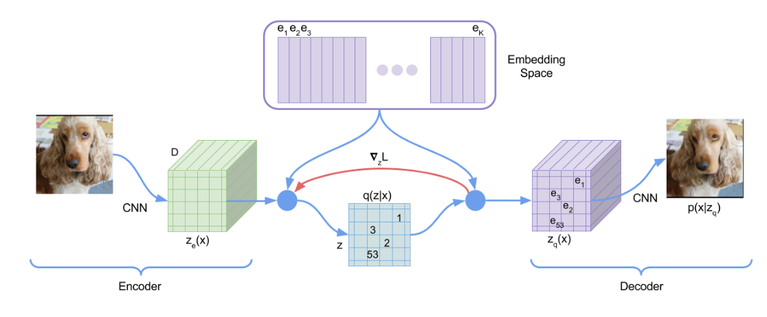
There are four components that are parametrized: the codebook embedding $e_{\theta}$, encoder $E_{\theta}$, and decoder $D_{\theta}$, and the priors $p_\theta$ over the embedding space. The codebook is $e_{\theta} \in \mathbb{R}^{K \times D}$. $K$ is the size of the codebook, and the $D$ is the code length for each of the embedding. $\theta$ denotes the entire set of parameters, which is learned through data. Note that the codebook is learned. The encoder is a neuralnet. It could be any neural network. 16 uses a CNN, but this is a design choice that could be experimented. The exact architecture is not required by theory but will greatly impact empirical results. The encoder takes an image, $x \in \mathbb{R}^{3 \times H \times W}$ as input, and outputs into the embedding space $\mathbb{R}^{D}$. The full dimensionality of this stage depends on the neuralnet architecture. For example, we could choose a $32 \times 32$ embedding vectors to represent an image of $128 \times 128$. This output is quantized and drop its embedding dimension $D$. Each embedding is quantized into a number $z \in \{1, ... K\}$. That is, each embedding vector is no longer a $D$-vector but just a number. Lastly, the decoder is another neuralnet that takes the quantized embedding and output an image in $\mathbb{R}^{3 \times H \times W}$. The prior $p_\theta$ is over the embedding space. It could be such that it is conditioned on some labels. That is, $p_\theta(z | l)$, where $l$ represents label classes. The prior allows us to sample an embedding based on a class label.

Image generation is straight forward. First, we sample encodings from the priors neural network $p_\theta(z|l)$. Second, the encodings are fed through the decoder network $D_{\theta}$ to generate an image. This methodology also applies well to music generation; see 6 . The only difference is that instead of $x$ representing an image, it represent an audio segment.

The key question is how to train these 4 components: $e_{\theta}, E_{\theta}, D_{\theta}, and p_{\theta}$. This is broken down into two stages. The first stage approximate $e_{\theta}, E_{\theta}, D_{\theta}$. Let’s write down the loss function associated with them:

\begin{equation} \mathscr{L}(x; \theta) = ||x - D_\theta()||_2^2 + ||sg[E_{\theta}(x)] - e_\theta||_2^2 + \beta ||sg[e_\theta] - E_\theta(x) ||_2^2 \end{equation}

Note that $D_\theta(x)$ is an abuse of notion to denote the generated image if we take the input as the quantized encoded embedding. The first term is the reconstruction loss, the second term is a simple vector quantization loss, and the third term is the commitment loss to ensure that embedding space does not grow too large. The goal here is not to explain how to derive or improve these loss terms, we want to know how to operationalize the training by using data. With this loss defined, it is now clear that all we have to do is to feed data into all the parametrized functions (e.g $e, E, D$), calculate the loss, and then perform gradient descent with each batch of data.

The second stage approximates priors’ probability distributions of the encodings, $p_{\theta}$. It might be tempting to model the density functions explicitly via log likelihood, cross-entropy, or other probability divergence measures. This approach is empirically useless because the dimensionality of embedding space is too large. One of the breakthrough in AI is the ability to model probabilistic model with autoregressive models, as evidenced and made hugely popular by the success of LLM. This technique applies here as well. The encodings are treated as any other high dimensional object, in this case $e = (e_1, e_2, ..., e_D)$. The model take a partial vector $(e_1, ... e_i)$ as input and predicts the next token $e_{i+1}$. The loss could be just a L2 loss between $(e_1, ... e_i, e_{i+1})$ and $(e_1, ... e_i, \hat{e}_{i+1})$. This simple setup allows us to update the neural network. The current state of the art uses neural networks that are transformer based.

See 2 , 5 , 4 , 10 for more details about estimating high dimension joint probability distribution. See 6 , 12 for details about more design space for vq-vae encode-decoder system.

Diffusion via Score Matching

One of the most popular image generating model is diffusion. We take a look at the model presented in 8 . $x$ is in the image space. There is a diffusion process $x_t \sim \mathscr{N}(x_{t-1}, I)$ such that, $x_0$ is the original image, and $x_t$ is the previous image $x_{t-1}$ plus some white noise. The generating model is the reverse of this process. We model this reverse process with a transition probability density. The transition process is represented as

\begin{equation} p_{\theta}(x_{t-1} | x_t) = \mathscr{N}(x_{t-1}; \mu_\theta(x_t, t), \sigma_\theta (x_t, t)) \end{equation}

For simplicity, we set $\sigma_\theta$ to be fixed and only focus on $\mu_\theta$. We would like to approximate $\mu_\theta$ using a neuralnet. Once we have that approximation, the generating process is as simple as just start with a white noise $x_T$, and then sample $x_{t-1}$ from $x_t$ based on the transition probability $p_\theta$. We repeat this transition for $T$ steps.

To approximate $\mu_\theta$, we rewrite and parse out a new quantity $\epsilon_{\theta}$, defined as

\begin{equation} \mu_{\theta}(x_t, t) = \frac{1}{\sqrt{\alpha_t}} \left[ x_t - \frac{\beta_t}{\sqrt{1- \bar{\alpha_t}}} \epsilon_{\theta}(x_t, t) \right] \end{equation}

A neuralnet is setup to represent $\epsilon_{\theta}$ and is optimized by training on this loss,

\begin{equation} \mathscr{L}(x_0, t; \theta) = || \epsilon - \epsilon_{\theta} ( \sqrt{\bar{\alpha_t}} x_0 + \sqrt{1- \bar{\alpha_t}} \epsilon, t) ||^2, \end{equation}

where $\epsilon \sim \mathscr{N}(0, I)$ and $t \sim U(1, ..., T)$, and $x_0$ is a data sample. The loss could be calculated for each data point. The complexity of this generating model is deriving what the neuralnet supposes to represent and the loss function. But when these entities are written out, it is relatively straight forward to understand the computations both in inference and training stage.

See 13 for an improved version of this diffusion model.

Diffusion via SDE

The diffusion process could be formulated as a stochastic process. This is my personal favorite because theory is compact and succinct. Let $\{ x_t \}_{t=0}^T$ be the forward diffusion process modeled as an Itô integral,

\begin{equation} dx = f(x, t)dt + g(t) d \mathbb{W}, \end{equation}

where $\mathbb{W}$ is a Wierner process. $f(x,t)$ is a drift term, and $g(t)$ quadratic variation. For simplicity, we set them to be time-dependent constants. The reverse process is a known math result, see 1 ,

\begin{equation} dx = \left[ f(x,t) - g(t)^2 \nabla_x \log p_t(x) \right]dt + g(t)dW, \end{equation}

where $dt$ is negative timestep and $W$ is a backward Wierner process. We can solve this backward SDE numerically if we know the term $\nabla_x \log p_t(x)$. We estimate $\nabla_x \log p_t(x)$ with a neuralnet. With that, we have a generating model because the reverse process is fully described by the backward SDE.

The neuralnet that needs to be learned from data is $s_{\theta}(x, t) := \nabla_x \log p_t(x)$, which 15 names the score function. It shows that this neural network could be efficiently trained by minimizing the objective

\begin{equation} \mathscr{L}(x, t; \theta) = \mathbb{E}_{p_{data}(x)} \left[ tr(\nabla_x s_{\theta}(x)) + \frac{1}{2} ||s_{\theta}(x) ||^2 \right] \end{equation}

The expectation is estimated by the batch average of training samples. There are additional techniques to training the score network that works with perturbed sample data; see 2 . 15 uses a random projection to approximate $tr(\nabla_x s_{\theta}(x))$. Regardless of training methods, the key is that $s_{\theta}$ is approximated by neuralnet that could be efficiently trained from data samples.

Diffusion via Continuous Normalizing Flows (CNFs)

The continuous normalizing flow formulation is slightly involved but a more general approach than other diffusion setups. We follow the notation in 9 . Let $\{ x_t \}_{t=0}^T$ be the series of transformation from noise to data. The time-dependent probability path governing this transformation is $p_t$. We define a time-dependent map $\phi_t$, which is called the flow,

\begin{eqnarray*} \frac{d}{dt} \phi_t(x) &=& v_t(\phi_t(x)) \\ \phi_0(x) &=& x \end{eqnarray*}

Then, $p_t$ is defined as,

\begin{equation} p_t = p_0 (\phi_t^{-1}(x)) \det \left[ \frac{\delta\phi_t^{-1}}{\delta x} \right] \end{equation}

The most important object is $v_t$, which is called the generating vector of the probability path. We approximate this vector by a neuralnet, $v_t(\theta)$. The ODE and $v_t(\theta) solve $\phi_t$, which lead to $p_t$. There are some traditional numerical methods to solve ODE, or we could use a neural ODE technique; see 3 . $p_t$ describes the transition probability of $x$.

Let’s describe how to estimate $v_t(\theta)$. Consider the flow matching objective,

\begin{equation} \mathscr{L}(x, t; \theta) = \mathbb{E}_{t, p_t(x)} ||u_t(x) - v_t(x; \theta) ||^2 \end{equation}

But we don’t know $p_t$ and $u_t$. Instead, we could switch to a conditional flow matching objective,

\begin{equation} \mathscr{L}(x, t; \theta) = \mathbb{E}_{t, q(x_0), p_t(x|x_0)} ||v_t(x; \theta) - u_t(x|x_0)||^2 \end{equation}

This loss leads to the same gradient with respect to $\theta$ as the flow matching objective. With this transformation, we can get a solid handle on $p_t(x|x_0)$, and indirectly the generating function $u_t(x|x_0)$. For example, we can consider a special, gaussian probability path,

\begin{equation} p_t(x|x_0) = \mathscr{N} (x | \mu_t(x_0), \sigma_t(x_0)) \end{equation}

It simply means that the transition is sampled from gaussian that has time-dependent mean and variance. This special flow leads to a rather simple form for $u_t(x|x_0)$

\begin{equation} u_t(x|x_0) = \frac{\sigma_t^{\prime}(x_0)}{\sigma_t(x_0)} ( x - \mu_t(x_0)) + \mu_t^{\prime} (x_0) \end{equation}

Let see how we update the parameters of the neuralnet representing $v_t(\theta)$. Take a batch of samples, the expectation is estimated over the sample batch. $u_t(x|x)$ is directly calculated. We get the conditional flow matching loss value, and then we can perform gradient descent on $\theta$.

The CNF formulation is a generalization of diffusion model, e.g. as described in 15 . This shows that even modeling the same generating process, we could approximate different components. 15 uses the neuralnet to represent a score function, and 9 approximates a time-dependent vector field.

GAN

GAN model was introduced by 7 . It uses two neural networks, a generator and a discriminator, to model a competitive game between the two neural networks. Take the example of a text-to-image GAN model. The generator neural network takes text as input and output image. The discriminator neural network takes input and image pair, and output a probability on if the image is real or fake. GAN models tend to be small in parameter size. They are are easy to use because sampling only requires running the generator neural network once to generate new samples.

Training a GAN model updates the two networks simultaneously. The discriminator loss function keep tracks of how well it could distinguish the fake and the real images given a text-image pair. The generator loss function keeps track of how well it could trick the discriminator. When we feed a batch of text-image pairs to the generators, we get fake images. We can use the text, real image, and fake images to calculate the loss for both of the discriminator and the generator networks, allowing for updates of both network’s parameters.

Autoregressive Model (DALLE)

Autoregressive model is made popular by GPT. An autoregressive model takes a token sequence as input and outputs one more token. The initial sequence and the predicted token form a new token sequence to be fed into the model again. This process repeats itself until the predicted token is a special STOP token. Training on an autoregressive objective is often called pre-training because raw data could be fed into the model directly. The raw data could be text, image, audio, or video. These data are encoded into token space as sequences, and each token sequences could be converted into multiple subsequences and the next token as the input and expected output for training. This paradigm works extremely well for text, the so called language models.

We can look at a specific example that deals with image, the dalle model described in 11 . It has two major components: the visual encoder-decoder system and the prior over text-image token sequence. The first component is similar to what we discussed in details in the VQ-VAE model. For discussion simplicity, we just assume that its encoder-decoder setup follows what is described there. The key difference lies in how dalle estimates the prior. The text is encoded by the BPE encoder, see 14 . This encoder is calculated from the corpus and does not require training a neural network. The text token length is padded to a fixed length of 256. The image is encoded by the visual encoder into the codebook space, which has dimension of $K$. The text and visual token sequences are concatenated to be used as input in the second component, an autoregressive model over the visual token space. The generating process starts with a text token sequence. It repeatedly generates the next token until the desired image token sequence length is reached. The image token sequence is then decoded into an image by the visual decoder.

The BPE encoder is calculated directly from the corpus. This algorithm is fast and efficient. The visual encoder-decoder follows similar steps as discussed VQ-VAE. This takes the form of multiple neural networks. The autoregressive neural network is trained on raw text-image pairs. The loss objective is how well the neuralnet predicts the next visual token. This is a technique to indirectly model the full probability distribution of the visual token space. It is an approach that is well demonstrated by LLM to approximate high dimension probability space. See 2 , 5 , 4 , 10 . The neural network in this components could be many orders of magnitude larger than the visual encoder system. The majority of the training resources is spent on training for an neural network to estimate a probability distribution.

Discussion

I have not said much about the internal architectures of the neural networks described in each example. It is a point that I want to make that the role of neural network is not required in theory. Any high dimension estimation methods could work. However, neural networks have become the only meaningful way to approximate high dimensional function in these models. As the writing of this post, these neural networks invariably use CNN and transformer components. I would expect that the internal architectures will evolve, and we might see new class of internal architectures as soon as in a few years.

One of the most important aspect of model formulations is deciding on what to estimate. This decision is usually guided by two factors. The approximated entity should be easy to use in the inference stage. For example, the inference of GAN model is much faster than a diffusion or an autoregressive token model. GAN model only needs to pass through the generating neuralnet once to get the result, but a diffusion step needs to be run $T$-many passes through the probability transition step.

The other aspect of formulation is the efficiency of learning from data. It is easy to spot an entity that is useful to estimate with a neural network. For the example of an image diffusion process, it is obvious that we want to estimate the time-dependent, joint distribution that governs the reverse process. In theory, we could generate sequence samples from raw images, and use them to approximate the transition directly. This is not going to lead to good empirical results. Instead, we have the somewhat convoluted diffusion models in the form of score matching, SDE, and CNF. Each of these models make additional assumptions about the reverse process to allow for clever math so that we could derive some entities that could be efficiently learned from data.

The learned models need to generalize well beyond sample data. The approximating neural network is trained on some loss objective. It is easy to get a neural network to fit the data well. The effectiveness of the model is not necessarily determined by this arbitrary loss objective, but on how well it performs for the intended generation task. The amazing thing about these deep learning techniques is that these tremendously large deep neural networks are able to acquire the ability to generalize to tasks that are not directly specified in the training data.

Footnotes

It is worth noting that some generative models does not contain any interpretable intermediate steps. It could be just one giant blackbox neural network model that transforms the text into an image. Human researchers might understand how individual computation is performed, but we might not able to make sense of any intermediate representations. ↩

Citations

van den Oord, Aaron, Vinyals, Oriol, and Kavukcuoglu, Koray. Neural discrete representation learning. 2018. URL: https://arxiv.org/abs/1711.00937, arXiv:1711.00937. ¹ ² ³
Dhariwal, Prafulla, Jun, Heewoo, Payne, Christine, Kim, Jong Wook, Radford, Alec, and Sutskever, Ilya. Jukebox: a generative model for music. 2020. arXiv:2005.00341. ¹ ²
Bengio, Yoshua, Yao, Li, Alain, Guillaume, and Vincent, Pascal. Generalized denoising auto-encoders as generative models. 2013. URL: https://arxiv.org/abs/1305.6663, arXiv:1305.6663. ¹ ² ³
Chen, Xi, Mishra, Nikhil, Rohaninejad, Mostafa, and Abbeel, Pieter. Pixelsnail: an improved autoregressive generative model. 2017. arXiv:1712.09763. ¹ ²
Chen, Xi, Kingma, Diederik P., Salimans, Tim, Duan, Yan, Dhariwal, Prafulla, Schulman, John, Sutskever, Ilya, and Abbeel, Pieter. Variational lossy autoencoder. 2017. URL: https://arxiv.org/abs/1611.02731, arXiv:1611.02731. ¹ ²
Radford, Alec, Wu, Jeffrey, Child, Rewon, Luan, David, Amodei, Dario, and Sutskever, Ilya. Language models are unsupervised multitask learners. 2018. URL: https://d4mucfpksywv.cloudfront.net/better-language-models/language-models.pdf. ¹ ²
Razavi, Ali, van den Oord, Aaron, and Vinyals, Oriol. Generating diverse high-fidelity images with vq-vae-2. 2019. arXiv:1906.00446. ¹
Ho, Jonathan, Jain, Ajay, and Abbeel, Pieter. Denoising diffusion probabilistic models. 2020. arXiv:2006.11239. ¹
Rombach, Robin, Blattmann, Andreas, Lorenz, Dominik, Esser, Patrick, and Ommer, Björn. High-resolution image synthesis with latent diffusion models. 2022. URL: https://arxiv.org/abs/2112.10752, arXiv:2112.10752. ¹
Anderson, Brian D O. Reverse-time diffusion equation models. Stochastic Process Application, 12(3):313–326, 1982. ¹
Song, Yang, Sohl-Dickstein, Jascha, Kingma, Diederik P., Kumar, Abhishek, Ermon, Stefano, and Poole, Ben. Score-based generative modeling through stochastic differential equations. 2021. URL: https://arxiv.org/abs/2011.13456, arXiv:2011.13456. ¹ ² ³ ⁴
Lipman, Yaron, Chen, Ricky T. Q., Ben-Hamu, Heli, Nickel, Maximilian, and Le, Matt. Flow matching for generative modeling. 2023. URL: https://arxiv.org/abs/2210.02747, arXiv:2210.02747. ¹ ²
Chen, Ricky T. Q., Rubanova, Yulia, Bettencourt, Jesse, and Duvenaud, David. Neural ordinary differential equations. 2019. URL: https://arxiv.org/abs/1806.07366, arXiv:1806.07366. ¹
Goodfellow, Ian J., Pouget-Abadie, Jean, Mirza, Mehdi, Xu, Bing, Warde-Farley, David, Ozair, Sherjil, Courville, Aaron, and Bengio, Yoshua. Generative adversarial networks. 2014. URL: https://arxiv.org/abs/1406.2661, arXiv:1406.2661. ¹
Ramesh, Aditya, Pavlov, Mikhail, Goh, Gabriel, Gray, Scott, Voss, Chelsea, Radford, Alec, Chen, Mark, and Sutskever, Ilya. Zero-shot text-to-image generation. 2021. URL: https://arxiv.org/abs/2102.12092, arXiv:2102.12092. ¹
Sennrich, Rico, Haddow, Barry, and Birch, Alexandra. Neural machine translation of rare words with subword units. 2016. URL: https://arxiv.org/abs/1508.07909, arXiv:1508.07909. ¹