From Zero to Cracking secp256k1 - A condense intro to Shor's

There has been some recent hype about quantum supremacy. There are talks about how there will be a commercial quantum system in the next 5 years. I have to get myself educated on this topic. Unlike my other posts, I do not have any personal experiences working on this topic. I am a practitioner on most other things I write about. On quantum computing, I am just a fan. This is a fun post for me to write. It forces me to spend time on the subject. I focus on answering the one question that interests me the most. How do we use quantum computing to crack secp256k1, the cryptographic system that underpins trillions of dollars of cryptocurrencies.

Preliminaries¶

Notation¶

Let $\mathbb{H}$ be a Hilbert space, and $\mathbb{H}^*$ be set of linear maps from $\mathbb{H} \mapsto \mathbb{C}$, where $\mathbb{C}$ denotes the complex number field. Elements in $\mathbb{H}$ is denoted by ket vector $|x \rangle$, and elements in $\mathbb{H}^*$ is denoted by bra vector $\langle y|$. And $\langle y|x \rangle \in \mathbb{C}$. For any $\langle x| \in \mathbb{H}^*$, it could be called the dual of $|x \rangle \in \mathbb{H}$, and $\langle y|x \rangle$ is an inner product of $|x \rangle$ and $ \langle y |$.

A $n$-qubit system is a $2^n$-dimensional Hilbert space. For a concrete example, let $\mathbb{H}$ be a 4 dimensional Hilbert space. The standard orthnormal basis in vector notation are:

$$ \begin{pmatrix} 1 \\ 0 \\ 0 \\ 0 \end{pmatrix}, \begin{pmatrix} 0 \\ 1 \\ 0 \\ 0 \end{pmatrix}, \begin{pmatrix} 0 \\ 0 \\ 1 \\ 0 \end{pmatrix}, \begin{pmatrix} 0 \\ 0 \\ 0 \\ 1 \end{pmatrix}. $$

In quantum mechanics and quantum computing, it is more convenient to use the bracket notation

$$ |00\rangle, |01\rangle, |10\rangle, |11\rangle $$

As we will see later, this is a convenient computing basis.

Quantum States¶

The state of quantum system is described by a vector in a Hilbert Space. For example, let’s pick the basis $|0\rangle$ and $|1 \rangle$ for a 1-qubit system. A state $\psi \in \mathbb{H}$ is a linear combination of the chosen basis,

$$ \alpha_0 |0\rangle + \alpha_1 |1\rangle, $$

where $\alpha_0, \alpha_1 \in \mathbb{C}$. The evolution of the state of a closed quantum system is described by a unitary operator. For any evolution, there is a unitary operator $U$ such that,

$$ |\psi_2\rangle = U |\psi_1\rangle. $$

A concrete example of a $1$-qubit system is using polarization states of a single photon to represent the quantum state. $|0 \rangle$ is horizontally polarized photon and $|1 \rangle$ is a vertically polarized photon. A $n$-qubit system could be constructed by composing $n$ many $1$-qubit system.

Quantum Gates and Circuit¶

Let’s look at a simple $1$-qubit quantum circuit.

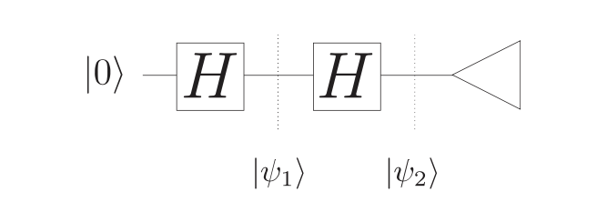
The circuit starts with the state $|0\rangle$. The $H$ operator is called the Hadamard gate, which will be explained shortly. The most basic operators are also called quantum gates because gates are the building blocks of more complex operators. The quantum state becomes $\psi_1$ after the Hadamard gate, which is $H |1\rangle = |\psi_1\rangle = \frac{1}{\sqrt{2}} |0\rangle + \frac{1}{\sqrt{2}} |1\rangle$. After second Hadamard gate, the state become $H \lvert \psi_1 \rangle = \lvert 0 \rangle$. This will be obvious once we write down what Hadamard gates are in algebraic notation.

The most basic gates unitary transformation are basic rotations:

$$ I \equiv \begin{bmatrix} 1 & 0 \\ 0 & 1 \end{bmatrix}, \quad X \equiv \begin{bmatrix} 0 & 1 \\ 1 & 0 \end{bmatrix} $$

$$ Y \equiv \begin{bmatrix} 0 & -i \\ i & 0 \end{bmatrix}, \quad Z \equiv \begin{bmatrix} 1 & 0 \\ 0 & -1 \end{bmatrix} $$

These transformations are called Pauli gates. $I$ is the identity operator. For example, $I |0 \rangle \langle = |0 \rangle$. The $X$, $Y$, and $Z$ corresponds to rotations if we look at the quantum state in the Bloch sphere, which is just kind of a polar coordinate system for $1$-qubit system. In particular $X$ is the NOT gate because $X |0 \rangle = |1 \rangle$. and $X |1 \rangle = |0\rangle$

In classical circuits, the set of { AND, OR, NOT } gates are universal because any logical function, such as addition, subtraction, and if-then logic, can be built using only these gates. In quantum circuits, $X$, $Y$, and $Z$ do not form a universal set. For one, they cannot encode entanglement. But there is a simple universal set. The set $\{H, T, CNOT \}$ is universal. $H$ is called the Hadamard gate,

$$ H = \frac{1}{\sqrt{2}} \begin{bmatrix} 1 & 1 \\ 1 & -1 \end{bmatrix}. $$

$T$ is known as the $\frac{\pi}{8}$-phase gate,

$$ T = \begin{bmatrix} e^{-i \frac{\pi}{8}} & 0 \\ 0 & e^{i \frac{\pi}{8}} \end{bmatrix}. $$

$CNOT$ is known as the controlled-not gate,

$$ CNOT = \begin{bmatrix} 1 & 0 & 0 & 0 \\ 0 & 1 & 0 & 0 \\ 0 & 0 & 0 & 1 \\ 0 & 0 & 1 & 0 \end{bmatrix}. $$

The controlled-not gate flips the state of the second qubit if the first qubit is $|1\rangle$ and does nothing if $0\rangle$. Note that $H$ and $T$ are $1$-qubit gate, but CNOT acts on 2 qubits. $H$ and $T$ cannot induce entanglement, but CNOT can. This is the main reason that pure rotation gates could not form a universal set.

Once we have a universal set, another key result is the Solovay–Kitaev Theorem, which states that we can approximate any unitary operator efficiently using only gates from a universal set. The existence of universal set and Solovay–Kitaev give us powerful tools to build quantum circuits.

Quantum Measurement¶

We can take a look at two circuits differing by only by an intermediate measure.

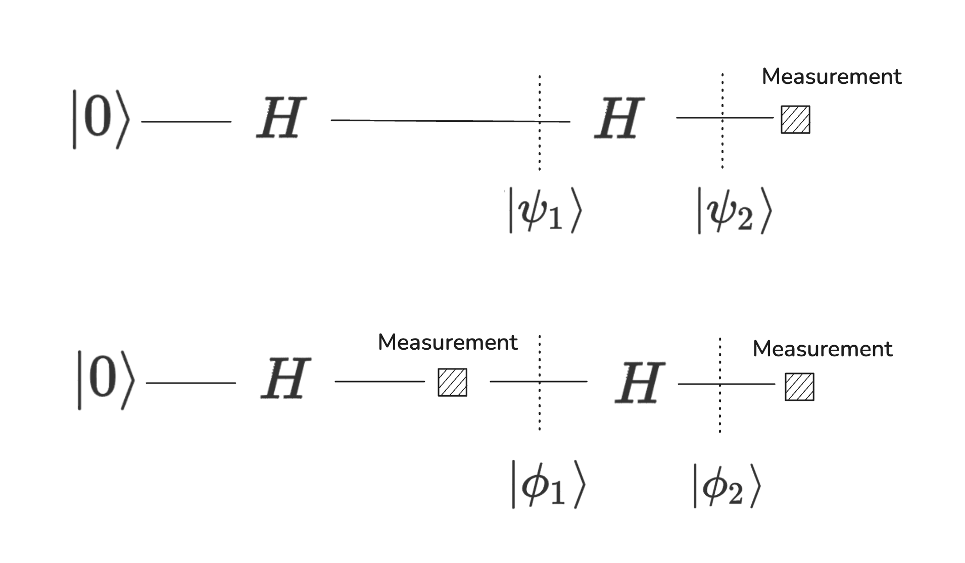
Measurement collapses the quantum state.

In the top circuit, the state right before the final measurement is $|0 \rangle$. The final measurement is always $0$. On the other hand, the bottom circuit has an extra intermediate measurement. This intermediate state $\phi_1$ is either $|0 \rangle$ or $|1 \rangle$, with equal probability. Then,

$$ |\phi_2\rangle = \begin{cases} \frac{1}{\sqrt{2}} (|0\rangle + |1\rangle) & \text{with probability } \frac{1}{2} \\ \frac{1}{\sqrt{2}} (|0\rangle - |1\rangle) & \text{with probability } \frac{1}{2}. \end{cases} $$

The final measurement of the second circuit will yield $0$ or $1$ with equal probability. The difference in the two circuits are due to an extra measurement.

Controlled Gate and Phase Kickback¶

We have seen a $\text{C}NOT$ gate, which is a conditional operation. The concept of control gate applies more generally to any unitary operation. This is usually drawn like the following.

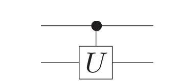
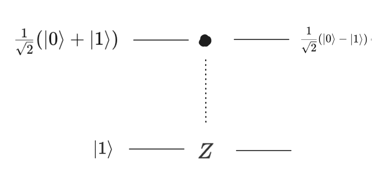
A controlled-$U$ gate, written as $\text{c-}U$.

In a 2-qubit system, it only acts on the one of the qubit and leave the other qubit untouched. Controlled gates are often used to implement a technique known as phase kickback, which is crucial to many quantum circuits. A controlled operation $U$ is applied to a target register while conditioning on a controlled register. Instead of affecting the target register, the control register experiences a phase shift. For example, in the following circuit, the $Z$ operation is controlled by the first qubit but the action is applied on the second qubit.

The final state is an entangled state $\frac{1}{\sqrt{2}} ( |0 1\rangle - |1 1\rangle )$. We can look at the control qubit marginally, and it is $\frac{1}{\sqrt{2}} (| 0\rangle - |1\rangle )$, which is just a phase shift of the initial control register. This is the magic of entanglement. It allows the phase information to be kicked back to the control register even though the action is intended to be on the target. The main algorithm will make use of this idea to encode key information in the frequency domain, and use phase kick back to extract the phase information.

First Look at the Discrete Log Circuit¶

We focus on the special case of the elliptical curve secp256k1, which I wrote about some years back in this post. The elements $a, b$ are group points as defined by the elliptical curve,

\begin{align*} B := \{ (x, y) \: | \: & y^2 = x^3 + 7 \; (mod \; p), \text{where } x,y \in \mathbb{F}_p \} \end{align*}

Unlike my previous blog, I am using multiplication to denote the group operation. The group operation of $P, Q, R \in B$ is such that $P \cdot Q \cdot R=0$ if all three points are aligned. We also set

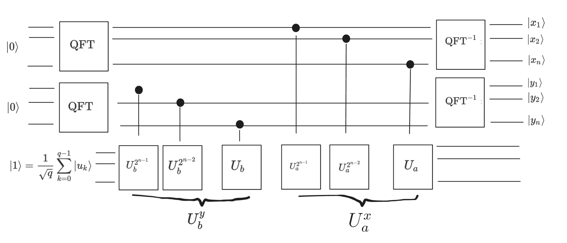
\begin{eqnarray*} p &=& 2^{256} - 2^{32} - 977 \\ q &=& 2^{256} - 2^{32} - 2^9 - 2^8 - 2^7 - 2^6 - 2^4 - 1. \end{eqnarray*}

$b^t$ means that $b \cdot b \cdots \cdot b$ for $t$-many times. It is just a notation. The problem statement is finding $t \in \{1, 2, \cdots, q\}$ for the discrete log problem $a = b^t$. In the case of public key cryptography, $a$ is the published public key and $t$ is the secret key. The goal is to find $t$ given the public key $a$. To solve this problem, we implement the following quantum circuit.

The circuit for solving the discrete log problem.

We use three registers. Each register uses $n=256$ qubit. The first two registers are called controlled registers, and the third is called target register. Applying the quantum operations of $\mathrm{QFT}$, $\mathrm{QFT}^{-1}$, $\text{c-}U^y_b$, and $\text{c-}U^x_a$, we measure the first two registers. We will cover the details of all these unitary operators in next section. We measure the first register to get a sequence of $x_i \in \{0, 1\}$. $\{x_1, \cdots, x_n\}$ are just a sequence of binary numbers, and it encodes a binary number $x$,

$$ x = 2^{n-1}x_1 + 2^{n-2}x_2 + \cdots + x_n = x_1 x_2 \cdots x_n. $$

$y$ is measured similarly. Now, calculate $\tilde{x} = \lfloor \frac{q \, x }{2^{256}} \rceil$ and $\tilde{y} = \lfloor \frac{q \, y }{2^{256}} \rceil$, and

$$ \tilde{t} = \frac{\tilde{y}}{\tilde{x}} $$

This $\tilde{t}$ has a good probability ($ \left[ \frac{8}{\pi^2} \right]^2 \approx 0.657$) to be the correct $t$ that solves the discrete log problem.

Notes that the circuit is tractable. The number of qubits required is in the order of $n=256$. The initiated quantum states are in the pure computational basis. We will unpack all these quantum operators $\mathrm{QFT}$, $\mathrm{QFT}^{-1}$, $\text{c-}U^y_b$, and $\text{c-}U^x_a$. We will show that they could be efficiently implemented.

Dissecting the Discrete Log Circuit¶

We will look at each of the key component that allows us to build up to the discrete log algorithm.

Step 1: QFT¶

The Discrete Fourier Transform (DFT) converts a sequence of complex numbers into another sequence of complex numbers. For example, if the original sequence just sampled the pressure of a sound wave, the transformed sequence corresponds to the amplitudes and phase of each of the frequency component. The two sequences contain the same information, but just in different computational basis.

The QFT is the unitary operator that maps each basis state $|x \rangle$ to a superposition of all basis states,

$$ \mathrm{QFT}: |x\rangle \;\mapsto\; \frac{1}{\sqrt{2^n}} \sum_{y=0}^{2^n - 1} e^{2\pi i \, \frac{x \, y}{2^n}} \;|y\rangle. $$

The transformation is a change of basis similar in spirit as in DFT. However, this operation is not a just a mathematical reformulation, it is a physical quantum evolution. Below is a circuit that implements the the QFT operation.

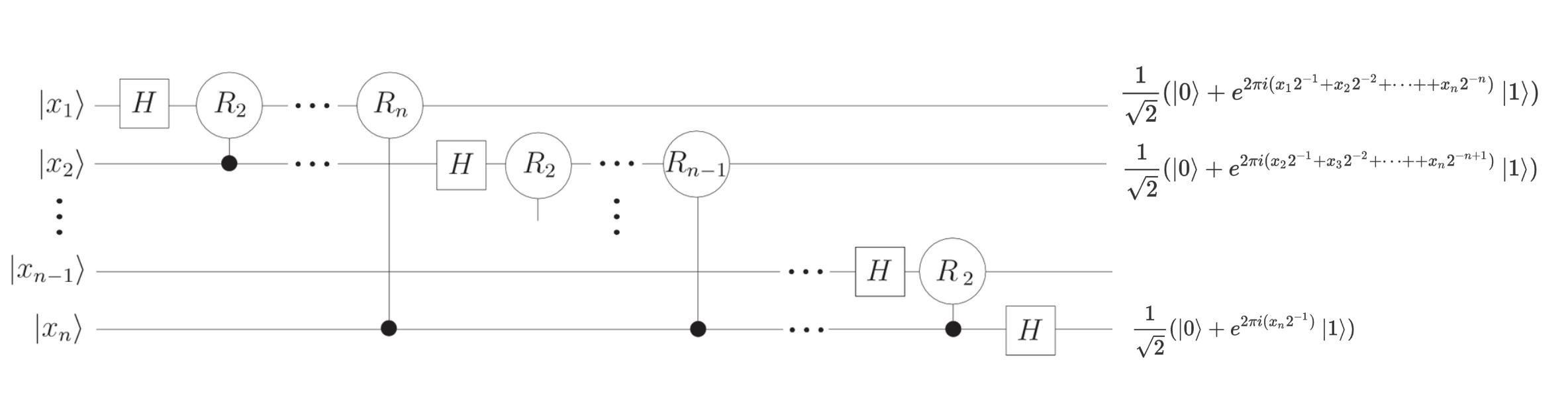
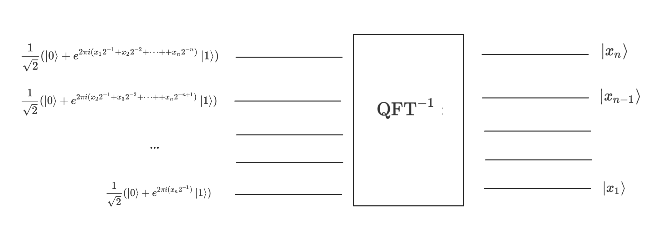
The $R_k$ operation is a $1$-qubit phase rotation operator, defined as

$$ R_k = \begin{pmatrix} 1 & 0\\ 0 & e^{\frac{2\pi i}{2^k}} \end{pmatrix}. $$

QFT is frequently used to create a convenient computational state of the quantum state. For example, we could first prepare the circuit to be in all $|0 \rangle$, and applying a $\mathrm{QFT}$ will give us a superposition state. Once we do some additional operations, we often want to convert the system back to th original computational basis for measurements. For that, we use $\mathrm{QFT}^{-1}$,

$$ \mathrm{QFT}^{-1} : |x\rangle \;\mapsto\; \frac{1}{\sqrt{2^n}} \sum_{y=0}^{2^n-1} e^{-2\pi i \frac{x\, y}{2^n} } \;|y \rangle. $$

The implementation of $\mathrm{QFT}^{-1}$ is just reversing the operation sequence of quantum gates and flip each quantum gates to its conjugate transpose.

Step 2: Phase Estimation¶

Let see how we can use $\mathrm{QFT}^{-1}$ to do phase estimation. We are given the quantum state $\frac{1}{\sqrt{2^n}} \sum_{y=0}^{2^n - 1} e^{2\pi i \,\omega\,y} \,|y\rangle$, we are asked to estimate $\omega$. Let’s rewrite omega as

$$ \omega = 2^{-1}x_1 + 2^{-2}x_2 + \cdots + 2^{-n} x_n, $$

then we can use the following circuit at $|x_n \rangle \cdots | x_1 \rangle$ and output $\{\tilde{x}_1, \cdots \tilde{x}_n \}$

Let $\tilde{x}= 2^n\omega=\tilde{x}_1 \tilde{x}_2 \cdots x_n$. It turns out that there is a $\frac{8}{\pi^2}$ probability that the true answer $\omega$ lies between $[\frac{x}{2^n}, \frac{x}{2^n}+1]$. The analytic constant $\frac{8}{\pi^2}$ is a bit mysterious. The phase estimation does not just cluster around the exact integer approximation $x$. It has non‐negligible support at $[x, x+1]$, where

$$ x= 2^n\omega = 2^{n-1}x_1 + 2^{n-2}x_2 + \cdots + x_n = x_1 x_2 \cdots x_n. $$

The accumulated probability is $\frac{8}{\pi^2}$.

It should be noted that this problem is a bit artificial because the input state of the circuit is prepared in some convenient superposition state. This algorithm is a component of the discrete log algorithm.

Step 3: Eigenvalue Estimation¶

The eigenvalue estimation algorithm is similarly artificial to phase estimation. But again, it is a building block toward the complete discrete log algorithm. The eigenvalue problem asks us to find $\omega$ given an arbitrary unitary operator $U$, its eigenstate $|\psi \rangle$, and the eigenvalue in the form of $e^{2\pi i \omega}$.

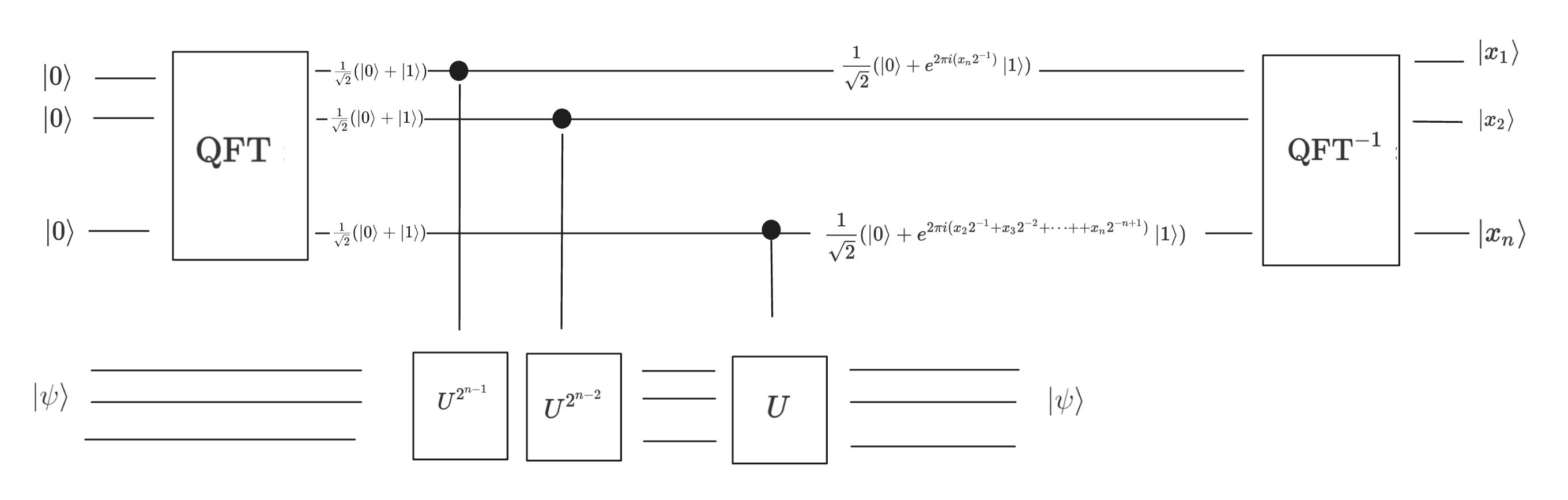
The circuit starts with input state $|0 \rangle$ and $\psi \rangle$. We measure $\{\tilde{x}_1, \cdots \tilde{x}_n \}$. Similar to the phase estimation, $\frac{\tilde{x}}{2^n}$ is a good estimate of $\omega$ with probability $\frac{8}{\pi^2}$. It is clear that the eigenvalue estimation problem is directly mapped to the phase estimation problem.

The operations on the bottom, target register is often denoted as $\text{c-}U^x$. This operation is effectively applying the unitary operator $x$ times. This operation kicks back the phase information to the control register. The $\mathrm{QFT}^{-1}$ operation decodes the phase information back to the computation basis for us to measure.

A key mystery of this circuit is how we could prepare the second register to be in some specific eigenstate $| \psi \rangle$. There is another clever technique that solves the problem for us via the Spectral Theorem. The theorem says that for any Hilbert space, there is an orthonormal basis consisting of only eigenvectors. This means that any state $\phi$ could be rewritten in the eigenvector basis

$$ |\phi\rangle = \sum_{j=0}^{2^n - 1} \alpha_j |\psi_j\rangle $$

If the starting state is arbitrary $\phi$ in the target register instead of eigenstate $|\psi \rangle$, the circuit maps the state to

$$ \sum_{j=0}^{2^n - 1} \alpha_j |\omega_j \rangle |\psi_j\rangle $$

The circuit map $|0\rangle^{\otimes n} |\psi_j\rangle$ to $|\omega_j \rangle |\psi_j\rangle$. Measuring the system collapse the system into an eigenstate $\psi_j$ with probability $|\alpha_j|^2$. This idea allows us use the eigenvalue estimation algorithm by preparing the target register in a convenient computational basis.

Step 4: Discrete Log One More Time¶

The eigenvalue estimation circuit is already very closely resembled the discrete log circuit. We have already explained in details $\mathrm{QFT}$, $\mathrm{QFT}^{-n}$. We need to explain $\text{c-}U_a^x$ and $\text{c-} U_b^y$.

Let’s define the unitary operator $U_a$,

$$ U_a : |s \rangle \mapsto | s \cdot a \rangle . $$

Note that the $\cdot$ denotes the elliptical group operation. This means that the binary number $s$ denotes a group element, but $| s \rangle$ is a quantum state, which could be pure state or a superposition state. $s \cdot a$ is again a group element. To apply the eigenvalue estimation algorithm we proposed earlier, we need to this operator’s eigenstate. The eigenstate is the following,

$$ |u_k\rangle = \frac{1}{\sqrt{q}} \sum_{s=0}^{q-1} e^{-2\pi i \frac{k}{q} s} |a^s \rangle. $$

We now have

\begin{eqnarray*} U_a |u_k\rangle &=& \frac{1}{\sqrt{q}} \sum_{s=0}^{q-1} e^{-2\pi i \frac{k}{q} s} U_a |a^s \rangle \\ &=& e^{2\pi i \frac{k}{q}} |u_k\rangle. \end{eqnarray*}

That is, $U_a$ has an eigenvalue of $e^{2\pi i \frac{k}{q}}$. Similarly, $U_b$ has an eigenvalue of $e^{2\pi i \frac{k t}{q}}$. If we have these two eigenvalues, $t$ is obvious. This is the reason why we did so much work to explain $\mathrm{QFT}$, phase estimation, and eigenvalue estimation. With just small amount of algebraic manipulation, we just converted the discrete log problem to problem of eigenvalue estimation.

The last thing we need is to show that we could prepare the target register of the discrete log circuit in the eigenvector state of $U_a$ and $U_b$. It turns out that all we need to do is to prepare the target register in $|1 \rangle$ because

\begin{eqnarray*} |0\rangle |1\rangle &=& |0\rangle \left( \frac{1}{\sqrt{q}} \sum_{k=0}^{q-1} |u_k\rangle \right) \\ &=& \frac{1}{\sqrt{q}} \sum_{k=0}^{q-1} |0\rangle |u_k\rangle. \end{eqnarray*}

That is the case because

\begin{eqnarray*} \frac{1}{\sqrt{q}} \sum_{k=0}^{q-1} |u_k\rangle &=& \frac{1}{\sqrt{q}} \sum_{k=0}^{q-1} \frac{1}{\sqrt{q}} \sum_{s=0}^{q-1} e^{-2\pi i \frac{k}{q} s} |a^s \rangle. \end{eqnarray*}

$a^s = | 1 \rangle$ if and only if $s = 0 \mod p$. Then $\frac{1}{\sqrt{q}} \frac{1}{\sqrt{q}} \sum_{k=0}^{q-1} e^{-2\pi i \frac{k}{q} \cdot 0} = \frac{1}{q} \sum_{k=0}^{q-1} 1 = 1$. It must be the case that all other states have amplitude $0$. The state $|0\rangle |1\rangle$ is the probably the friendliest to physical implementation.

Now we have the full discrete log circuit.

We prepare two control registers in $|0 \rangle$ and the target register in $|1 \rangle$. The $U_a$ and $U_b$ have the same eigenvector with slightly different eigenvalues. In fact, once we find out those eigenvalues, we can easily recover the secret key $t$. We first use $\mathrm{QFT}$ to convert the controlled registers into superposition state in the frequency domain. We use the control operations to kickback the eigenvalue to the controlled registers. We use $\mathrm{QFT}^{-1}$ to extract the eigenvalues. Voila! We just cracked the key cryptographic system that powers Bitcoin and Ethereum.

Not There Yet¶

All the theories are in place to implement circuits that allow us to find the private key for a Bitcoin account. Why is it the case that Bitcoin is still perfectly safe for the foreseeable future?

The most important quantum operation to implement is $U_b$. At a minimum, it requires circuits that perform elliptical curve point binary operations. Assume that we only use the universal set $\{H, T, CNOT\}$. All the modular arithmetic operations are on $n=256$ bit numbers. Implementing the group operation requires modular multiplication and inversion. We could estimate that $10^7$ gates are required for a single group point operation. Extrapolating this out in our circuit, we need at least $10^{9}$ quantum gates.

The most powerful quantum computer could handle 1000s of qubits. However, the maximum gate depth is more like 100s of gates. We need billions of gates. A key blocker is that qubits lose information over time due to decoherence. If the gate depth exceeds the coherence time, qubits lose their quantum states before the computation finishes.

The other key challenge to a feasible discrete log circuit is quantum error. Classical computing also has to deal with errors. However, the problem there is much less pronounced. For a typical consumer CPU, per bit-hour error rate is probably $10^{-10}$ to $10^{-18}$. Per operation rate would be $10^{-25}$. On the other hand, quantum per-qubit gate error rate is estimated to be $10^{-3}$. The comparison between the two systems is not just a problem of order of magnitude, it is order of order of magnitude. Even though our circuit only requires 1000 logical qubits, it requires at least millions of physical qubits if we were to implement any feasible error correction scheme. If we take the gate depth requirement into consideration, the quantum circuit will even much more complex.

In short, the current generation quantum computer is still many orders of magnitude short of being able to solve a discrete log problem associated with Bitcoin and Ethereum.

Intuition Behind the Quantum Speedup¶

There are many interpretations that explain why quantum computers is able to lead to speed up that classical algorithms cannot. I will highlight a few reasons that make the most sense to me.

Superposition offers the most basic yet intuitive explanation. We can compare $n$-qubit to $n$ classical bit. Let us revisit the definition of a quantum state. A $n$-qubit represents an element of Hilbert space with $2^n$ dimension. It is a $2^n$ dimensional vector. On the other hand, $n$ classical bit is only a $n$ dimensional vector. My favorite way to think about this is that a $n$-qubit quantum state represents a random variable whose set of events is $\Omega = \{ 0, 1\} ^n$. With the following quantum state,

$$ \psi\rangle = \sum_{i=0}^{2^n -1} \alpha_i |i\rangle, $$

it defines a random variable

$$ P(i) = |\alpha_i|^2, \quad \sum_{i=0}^{2^n -1} P(i) = 1. $$

But $n$-bit could only represents a single realization. The set of $\{ \alpha_i\}_i$ has cardinality of $2^n$. If we use $16$ classical bit to encode one $\alpha_i$, it would require $16 \cdot 2^n$ bits to encode the entire random variable. Superposition allows $n$ qubits to takes on simultaneous $2^n$ different possibilities. Quantum reality is tripping!

I find the quantum phenomenon of interference and entanglement to be less obvious in terms of how they immediately lead to speedup. To me, they are just basic quantum properties that govern the math behind quantum operators. However, if we have to hold on to them and come up with some intuitions, I think about inference as a technique that we could use to design our quantum algorithms to amplify the correct answers while allowing wrong answers to cancel each other out. Entanglement allows local operations to manipulate the entire quantum state collectively. In the mechanism of a phase kickback, entanglement makes the operation on a target register non-local, forcing a phase shift in the control register even though the quantum operation is explicitly performed only on the target register.

From Zero to Cracking secp256k1
A condense intro to Shor's